Friday, 24 May 2019

Power Factor Improvement

Power Factor Improvement

If the power factor is low or poor, it is necessary to improve or correct it. It may be improved by injecting a leading current into the circuit so as to neutralize the effect of lagging current. The power factor may be improved by using static capacitors or synchronous motors.

Power factor correction by static capacitors

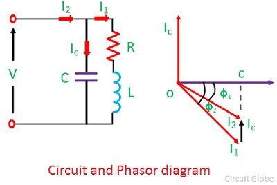
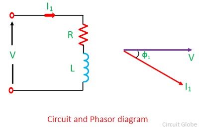
Consider an inductive load consisting of a resistor R and an inductor L connected to an AC supply. The circuit and phasor diagrams are shown in the figure.
power-factor-improvemet-1Let,
V – supply voltage.
I1 –  load current
φ1 – phase angle by which the current I1 lags behind the voltage
cosφ1 – original power factor
Let the capacitor C be placed in parallel with the load. It will take a leading current  I from the supply. The circuit and phasor diagrams are shown in the figure.
power-factor-improvement-2
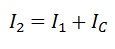
The total I2 drawn from the supply will be equal to the phasor sum of I1 and Icthat is

power-factor-improvement-equation-1Conclusions

  • The phase angle of I2 is φ2. It is seen from the phasor diagram that the φis less than φ1, and hence, cosφ2 is greater than cosφ1. In other words, the power is improved from cosφ1 to cosφ2.
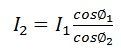
  • The new current supply from the supply is less than the load current I1, i.e., I2> I1. The new current is given by the equation
power-factor-improvement-3
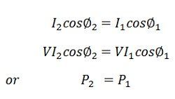
  • By connecting a capacitor in parallel with an inductive load, the power factor is improved, and the current from the supply is reduced without altering either current or power taken by the load.
power-system-improvement-3This relation shows that the power taken from the supply has not altered.

Static VAR Compensator

Static VAR Compensator

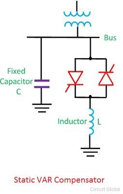
A static VAR compensator is a parallel combination of controlled reactor and fixed shunt capacitor shown in the figure below. The thyristor switch assembly in the SVC controls the reactor. The firing angle of the thyristor controls the voltage across the inductor and thus the current flowing through the inductor. In this way, the reactive power draw by the inductor can be controlled.
static-var-compensator-compressor(1)The SVC is capable of step less adjustment of reactive power over an unlimited range without any time delay. It improves the system stability and system power factor. Most commonly used SVC scheme are as follows.
  1. Thyristor controlled reactor (TCR)
  2. Thyristor-switched capacitor (TSC)
  3. Self Reactor (SR)
  4. Thyristor controlled reactor – Fixed capacitor (TCR-FC)
  5. Thyristor-switched capacitor – Thyristor controlled reactor (TSC-TCR)

Advantage of Static VAR Compensator

  • It increased the power transmission capability of the transmission lines.
  • It improved the transient stability of the system.
  • It controlled the steady state and temporary overvoltages.
  • It improved the load power factor, and therefore, reduced line losses and improved system capability.
Static VAR compensator has no rotating parts and is employed for surge impedance compensation and compensation by sectionalizing a long transmission line.

Methods of Voltage Control in Power System

Methods of Voltage Control in Power System

The voltage of the power system may vary with the change in load. The voltage is normally high at light load and low at the heavy-load condition. For keeping the voltage of the system in limits, some additional equipment requires which increase the system voltage when it is low and reduces the voltage when it is too high. The following are the methods used in the power system for controlling the voltage.
  1. On – Load Tap Changing Transformer
  2. Off – Load Tap Changing transformer
  3. Shunt Reactors
  4. Synchronous Phase Modifiers
  5. Shunt Capacitor
  6. Static VAR System (SVS)
Controlling the system voltage by the help of shunt inductive element is known as shunt compensation. The shunt compensation is of two types, i.e., the static shunt compensation and the synchronous compensation. In static shunt compensation, the shunt reactor, shunt capacitor and static VAR system are used, whereas the shunt compensation uses the synchronous phase modifier. The methods used for controlling the voltage are explained below in details.
1. Off – Load Tap Changing Transformer – In this method, the voltage is controlled by changing the turn ratio of the transformer. The transformer is disconnected from the supply before changing the tap. The tap changing of the transformer mostly done manually.
2. On – Load Tap Changing Transformer – This arrangement is used for changing the turn ratio of the transformer for regulating the system voltage when the transformer delivers the load. Most of the power transformer is provided with on-load tap changer.
3. Shunt Reactor – The shunt reactor is the inductive current element which is connected between the line and neutral. The shunt reactor compensates the inductive current from the transmission line or underground cables. It is mainly used in the long distance EHV and UHV transmission lines for reactive power control.
The shunt reactors are used in the sending end substation, receiving end substation and in the intermediate substation of long EHV and UHV line. In the long transmission line, the shunt reactor is connected at the distance of 300 Km to limit the voltage at an intermediate point.
4. Shunt Capacitors – The shunt capacitors are the capacitors connected in parallel with the line. It is installed at the receiving end substation, distribution substations and in the switching substations. The shunt capacitor injected the reactive volt-ampere to the line. It is placed in the three phase bank.
5. Synchronous Phase Modifier – The synchronous phase modifier is the synchronous motor running without a mechanical load. It is connected with the load at receiving the end of the line. The synchronous phase modifier absorbs or generates the reactive power by varying the excitation of the field winding. It keeps the voltage constant at any condition of the load and also improves the power factor.
6. Series Var Systems (SVS) – The static VAR compensator inject or absorb the inductive VAR to the system when the voltage becomes higher or lower than the reference value. In static VAR compensator, the thyristor is used as switching device in place of circuit breakers. Nowadays, the thyristor switching is used in the system in place of mechanical switching because thyristor switching is faster and provides transient free operation by controlling the switching.

Magnetic Hysteresis

Magnetic Hysteresis

The phenomenon of flux density B lagging behind the magnetizing force H in a magnetic material is known as Magnetic Hysteresis. The word Hysteresis is derived from the Greek word Hysterein means to lag behind. In other words, when the magnetic material is magnetized first in one direction and then in the other direction, completing one cycle of magnetization, it is found that the flux density B lags behind the applied magnetization force H.
There are various types of magnetic materials such as paramagnetic, diamagnetic, ferromagnetic, ferromagnetic and antiferromagnetic materials. Ferromagnetic materials are mainly responsible for the generation of the hysteresis loop.
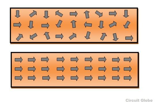
ferromagnetic-materialWhen the magnetic field in not applied the ferromagnetic material behaves like a paramagnetic material. This means that at the initial stage the dipole of the ferromagnetic material is not aligned, they are randomly placed. As soon as the magnetic field is applied to the ferromagnetic material, its dipole moments align themselves in one particular direction as shown in the above figure, resulting in a much stronger magnetic field.
Contents:
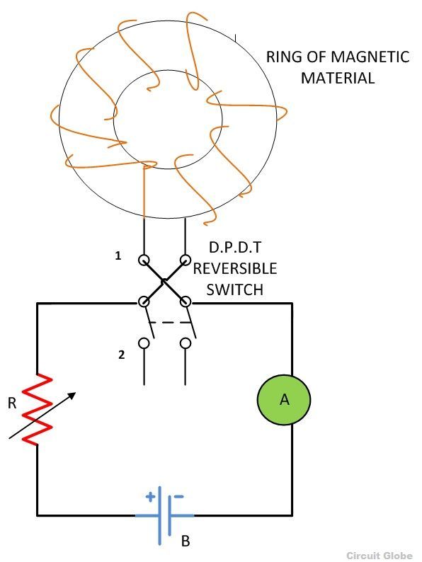
For understanding the phenomenon of the magnetic hysteresis, consider a ring of magnetic material wound uniformly with solenoid. The solenoid is connected to a DC source through a Double pole double throw (D.P.D.T) reversible switch as shown in the figure below
hysteresis-loop-circuit-diagram
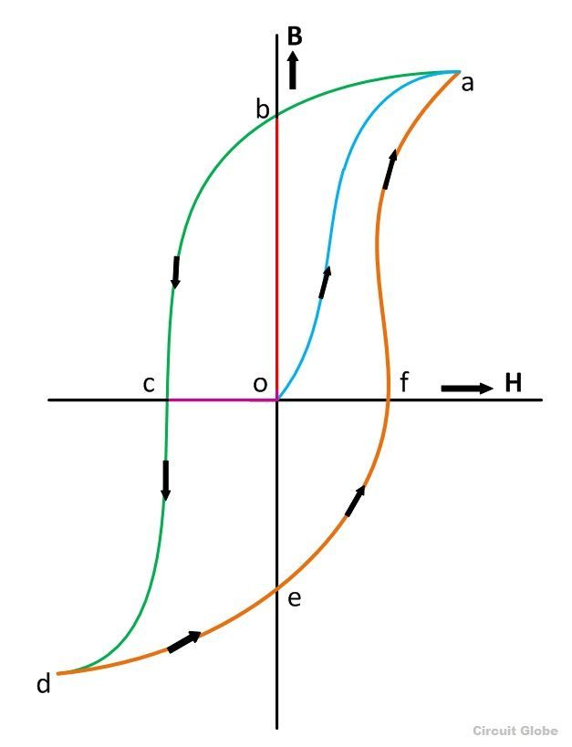
Initially, the switch is in position 1. By decreasing the value of R the value of the current in the solenoid increases gradually resulting in a gradual increase in field intensity H, the flux density also increases till it reaches the saturation point a and the curve obtained is oa. Saturation occurs when on increasing the current the dipole moment or the molecules of the magnet material align itself in one direction.
Now by decreasing the current in the solenoid to zero the magnetizing force is gradually reduced to zero, but the value of flux density will not be zero as it still has the value ob when H=0, so the curve obtained is ab as shown in the figure below.This value ob of flux density is because of the residual magnetism.
magnetic-hysteresis-loop

Residual Magnetism

The value of the flux density ob retained by the magnetic material is called residual magnetism, and the power of retaining it is known as Retentivity of the material.
Now to demagnetize the magnetic ring, the position of the D.P.D.T reversible switch is changed to position 2 and thus, the direction of flow of the current in the solenoid is reversed resulting in reverse magnetizing force H. When H is increased in reverse direction, the flux density starts decreasing and becomes zero (B=0) and the curve shown above follows the path bc. The residual magnetism of the material is removed by applying the magnetizing force known as Coercive force in the opposite direction.

Coercive Force

The value of the magnetizing force oc required to wipe out the residual magnetism ob is called Coercive force shown by pink color in the hysteresis curve shown above.
Now to complete the hysteresis loop the magnetizing force H is further increased in the reverse direction till it reaches the saturation point d but in the negative direction, the curve traces the path cd. The value of H is reduced to zero H=0 and the curve obtains the path de, where oe is residual magnetism when the curve is in the negative direction.
The position of the switch is changed to 1 again from the position 2 and the current in the solenoid is again increased as done in the magnetization process and due to this H is increased in the positive direction tracing the path as efa, and finally the hysteresis loop is complete. In the curve again of is the magnetizing force, also known as the Coercive force required to remove the residual magnetism oe.
Here the total Coercive force required to wipe off the residual magnetism in one complete cycle is denoted by cf. From the above discussion, it is clear that the flux density B always lags behind the magnetizing force H. Hence the loop ‘abcdefa’ is called the Magnetic Hysteresis loop or Hysteresis Curve.
Magnetic hysteresis results in the dissipation of wasted energy in the form of heat. The energy wasted is proportional to the area of the magnetic hysteresis loop. Mainly there are two types of magnetic material, soft magnetic material and hard magnetic material.

Soft magnetic material
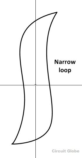
The soft magnetic material has a narrow magnetic hysteresis loop as shown in the figure below which has a small amount of dissipated energy. They are made up of material like iron, silicon steel, etc.
soft-magnetic-material-loop
Soft Magnetic Material Loop
  • It is used in the devices that require alternating magnetic field.
  • It has low coercivity
  • Low magnetization
  • Low retentivity

Hard magnetic material
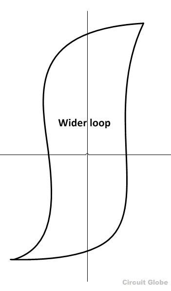
The Hard magnetic material has a wider hysteresis loop as shown in the figure below and results in a large amount of energy dissipation and the demagnitisation process is more difficult to achieve.
hard-magnetic-material
Hard Magnetic Material Loop
  • It has high retentivity
  • High coercivity
  • High saturation

Applications of Magnetic Hysteresis
  • Magnetic material having a wider hysteresis loop is used in the devices like magnetic tape, hard disk, credit cards, audio recordings as its memory is not easily erased.
  • Magnetic materials having a narrow hysteresis loop are used as electromagnets, solenoid, transformers and relays which require minimum energy dissipation.
Parallel Magnetic Circuit

Parallel Magnetic Circuit

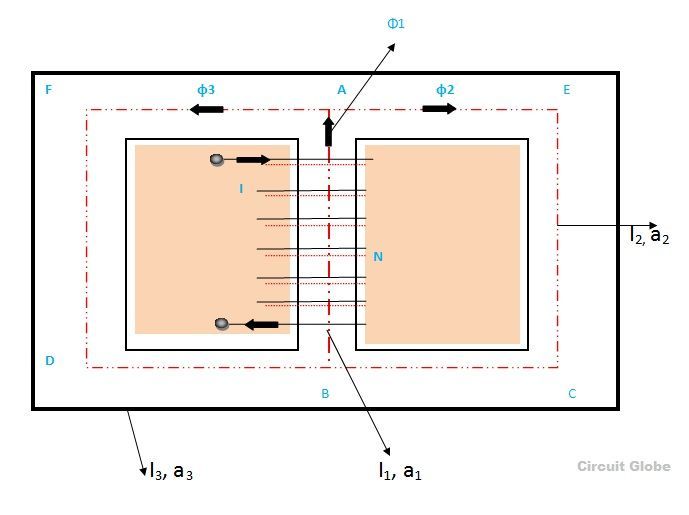
Definition: A magnetic circuit having two or more than two paths for the magnetic flux is called a parallel magnetic circuit. Its behavior can be compared to the parallel electric circuit.The parallel magnetic circuit contains different dimensional areas and materials having various numbers of paths.
PARALLEL-MAGNETIC-CIRCUIT1
The above figure shows parallel magnetic circuit. In this circuit, a current carrying coil is wound on the central limb AB. This coil sets up the magnetic flux φ1 in the central limb of the circuit. The flux φ1 which is in the upward direction is further divided into two paths namely ADCB and AFEB. The path ADCB carries flux φ2, and the path AFEB carries flux φ3. It is clearly seen fro the above circuit that
φ= φ2 + φ3
The two magnetic paths ADCB and AFEB forms the parallel magnetic circuit, thus, the ampere turns (ATs) required for this parallel circuit are equal to the ampere turns (ATs) required for any one of the paths.
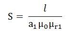
As we know, reluctance is
parallel-mag-ckt-eq-1
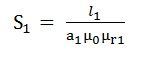
If S1 = reluctance of path BA will be
parallel-mag-ckt-eq2
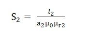
S=reluctance of path ADCB will be
parallel-mag-ckt-eq3
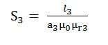
S3 = reluctance of the path AFEB will be
parallel-mag-ckt-eq4
Therefore, the total MMF or the total Ampere turns required in the parallel magnetic circuit will be the sum of all the individual parallel paths.
Total mmf required = mmf required for the path BA +mmf required for the path ADCB + mmf required for the path AFEB
parallel-mag-ckt-eq5
Where φ1. Φ2, φ3 are the flux and S1, S2, S3 are the reluctances of the parallel path BA, ADCB and AFEB respectively.

Series Magnetic Circuit

Series Magnetic Circuit

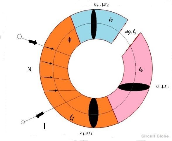
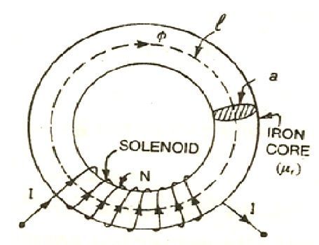
Definition: The Series Magnetic Circuit is defined as the magnetic circuit having a number of parts of different dimensions and materials carrying the same magnetic field. Consider a circular coil or solenoid having different dimensions as shown in the figure below
series-magnetic-circuit
Current I is passed through the solenoid having N number of turns wound on the one section of the circular coil. Φ is the flux, sets up in the core of the coil.
a1, a2, a3 are the cross-sectional area of the solenoid.
l1, l2, l3 are the length of the three different coils having different dimension joined together in series.
µr1, µr2, µrare the relative permeability of the material of the circular coil.
aand are the area and the length of the air gap.
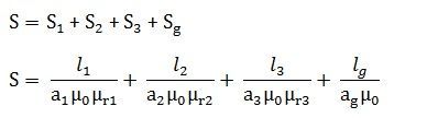
The total reluctance (S) of the magnetic circuit is
series-magnetic-circuit-eq1
Total MMF = φ x S ……..…. (1)

Series Magnetic Circuit

Definition: The Series Magnetic Circuit is defined as the magnetic circuit having a number of parts of different dimensions and materials carrying the same magnetic field. Consider a circular coil or solenoid having different dimensions as shown in the figure below
series-magnetic-circuit
Current I is passed through the solenoid having N number of turns wound on the one section of the circular coil. Φ is the flux, sets up in the core of the coil.
a1, a2, a3 are the cross-sectional area of the solenoid.
l1, l2, l3 are the length of the three different coils having different dimension joined together in series.
µr1, µr2, µrare the relative permeability of the material of the circular coil.
aand are the area and the length of the air gap.
The total reluctance (S) of the magnetic circuit is
series-magnetic-circuit-eq1
Total MMF = φ x S ……..…. (1)
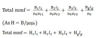
Putting the value of S in equation (1) we get
series-magnetic-circuit-eq2(As B = φ/a) putting the valve of B in the equation (2) we obtain the following equation for the total MMF
series-magnetic-circuit-eq3
Procedure for the Calculation of the total MMF for the Series Magnetic Circuit
  1. The magnetic circuit is divided into a different section or parts.
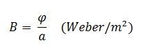
  2. Now determine the value of the flux density (B) of the different sections. As we know B = φ/a where φ is the flux in Weber, and a is the area of cross-section in m2
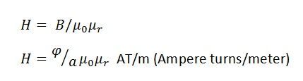
  3. Determine the value of the magnetising force (H) as we know that H = B/µ0µwhere B is the flux density in Weber/ m2 and µ0 is absolute permeability and its value is 4πx10-7, and µis the relative permeability of the material, and its value will be given. If the value of µr is not given, then you have to compute the value from the value of H from the B-H curve
  4. The value of magnetising force (H) as H1, H2, H3, Hg will be individually multiplied by the length of the different sections that is, l1, l2, l3 and lg respectively.
  5. Finally, add all the values of Hx l and therefore, the total MMF will be
series-magnetic-circuit-eq4
The value of H for the air gap part will always µg = B/µ0.
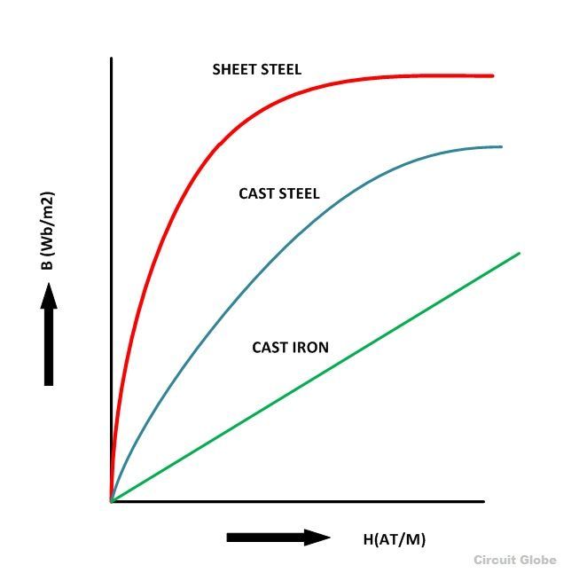
B-H Curve
The graph plotted between the flux density (B) and the magnetising force (H) of any material is called B-H Curve or the magnetisation curve.
The shape of the B-H curve is mostly non-linear this means that the relative permeability (µr) of the material varies and is not constant. The value of relative permeability mainly depends on the value of flux density. But for the non-magnetic materials like plastic, rubber, etc. and for the magnetic circuit having an air gap, its value is constant, denoted by (µ0). Its value is 4πx10-7H/m and commonly known as absolute permeability or permeability of free space.
B-H curve for the various material like cast iron, cast steel and sheet steel is shown below.
B-H-curve

Magnetic Circuit

Magnetic Circuit

The closed path followed by magnetic lines of forces is called magnetic circuit. In the magnetic circuit, magnetic flux or magnetic line of forces starts from a point and ends at the same point after completing its path. Flux is generated by magnets; it can be permanent magnet or electromagnets.
magnetic circuit is made up of magnetic materials having high permeability such as iron, soft steel, etc. Magnetic circuits are used in various devices like the electric motor, transformers, relays, generators galvanometer, etc. Consider a solenoid was having N turns wound on an iron core. The magnetic flux of ø Weber sets up in the core when the current of I ampere is passed through a solenoid.
Magnetic-circuit
Let, l = mean length of the magnetic circuit
A = cross-sectional area of the core
µr =  relative permeability of the core
Now the flux density in core material
mag-ckt-eq-1
Magnetising force in the core
magnetic-ckt-3-
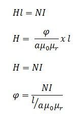
According to work law, the work done in moving a unit pole once round the magnetic circuit is equal to the ampere turns enclosed by the magnetic circuit.
mag-ckt eq 2
The above equation explains the following points
  1. Directly proportional to a number of turns (N) and current (I). It shows that the flux increase if the number of turns or current increases and decreases when either of the two quantity decreases. NI is the magnetomotive force (MMF).
  2. Inversely proportional to l/a µ0µrwhere (l/a µ0µr) is known as reluctance. The lower will be the reluctance the higher will be the flux and vice- verse.

Advantages of 3 Phase Over Single Phase System

Advantages of 3 Phase Over Single Phase System The three-phase system has three live conductors which supply the 440V to the large consu...